Advanced Model Update And Passage Relevance
Answer Extraction
What We Are Trying
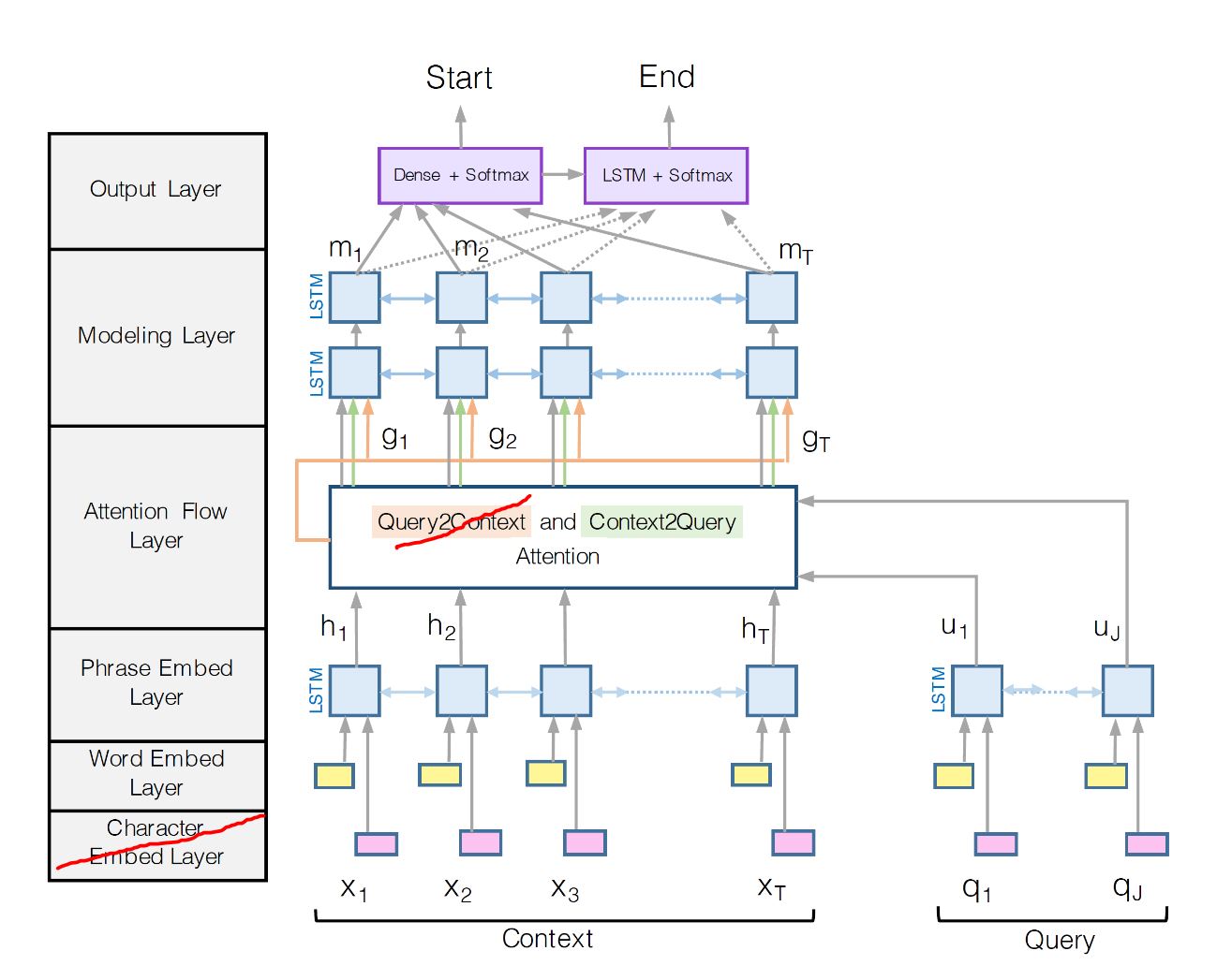
This week we decided to extend our attention model to implement the BiDAF model. BiDAF is a model designed by Minjoon, et al., and it performed very well in the squad dataset. So, we are trying to implement some of the aspects of BiDAF and see how it performs with the MS MARCO dataset. The BiDAF model (shown in the figure below) consists of six layers. Over the last week we implemented four layers fully and one layer partially. In specific, we implemented the Output Layer, the Modeling Layer, the Phrase Embed Layer, and the Word Embed Layer. Also, we implemented the Context2Query part of the Attention Flow Layer. The Context2Query attention layer signifies what query words are most relevant to different context words. We tried this model with new set of hyper-parameters similar to that in the paper and with the AdaDelta optimizer instead of the Adam optimizer. As for now, the model does not show improvement over the last attention model. We trained with a batch size of 64 and a learning rate of 0.3 and got these results:
| Metric | BiDAF (incomplete) |
|---|---|
| Bleu-1 | 0.494 |
| Bleu-2 | 0.474 |
| Bleu-3 | 0.462 |
| Bleu-4 | 0.440 |
| Rouge-L | 0.560 |
Next Steps
The next step for us definitely includes implementing the rest of BiDAF. For now we may not add char embedding, but we will definitely work on adding the Query2Context attention. The Query2Context attention signifies what context words have the closest similarity to the query words, which we expect to improve the accuracy of our model. We also did not have much time for hyperparameter tuning, so we hope to do this as well once we finish the model.
References
Seo, Minjoon, et al. “Bidirectional Attention Flow for Machine Comprehension.” arXiv preprint arXiv:1611.01603 (2016).
Passage Relevance
What We Are Trying
The biggest unanswered question we have right now in our model is how to handle passage relevance. For each sample, we are given an average of 8.21 passages averaging 421.68 characters. Sometimes only one of these passages are relevant, sometimes they all are. The dataset supplies an ‘is_selected’ attribute for each passage to tell if that passage was used to produce the answer. For each sample, an average of 1.07 passages are selected.
With all this, we have a few options of how to deal with passage relevance. The first question is do we concatenate the passages? We could concatenate all the passages or just a select few after another model filters out irrelevant passages. The issue with this is that we would have to train quite a large model and so training may be expense and have a tough time converging.
Another question to consider is do we use a model to pick which passages are relevant, and then send those passages in and not the others. An issue with this is that we would have to have a trustworthy passage selector to not throw out the answer along with the passage at this step. An alternative to this strategy that would alleviate this worry would be to simply rank the passages. This way we do not discard any information, but are able to focus the model on certain passages more than other based on the output from a separately trained model, acting almost as an attention mechanism. This would require some sort of method of picking the best answer out of a group of weighted answers in the end, not just picking the answer from the highest ranked passage.
The final question we are considering is to go neural or not. With the issue of passage relevance, we could use almost the same model as the answer extractor, just by switching the output to produce a single relevance number instead of two indexes in the text. A much simpler approach would be to use a non-neural model, whether it uses hand crafted features or even the GloVe embedding somehow.
So for this first attempt at passage relevance, we tried building both a neural model, based on our baseline answer extractor, and a non-neural model.
Because of the class imbalance between the selected and unselected passages, we were struggling to train a binary classifier. In response we put more weight on false negatives than on false positives in the loss function, and to not just converge on predicting not selected on every passage. But since the answer was often in many passages although just one was selected, the model had a tough time classifying the passages without a clear pattern in the training data. In response, we decided to stick with a ranking model versus a classification one.
An issue we ran into with any supervised model, neural or not, was what should the output be? All we have is if the passage is selected or not. Other than that we do not have any sort of ranking metric. In addition to this, sometimes the selected passage was not necessarily the best passage to find the answer anyway. Since it would be tough to frame a machine learning model with the data we had, we decided to stick with a ranking strategy that did not rely on training/learning.
This is where the TF-IDF statistic comes in. Term frequency-inverse document frequency is a statistic meant to reflect the importance of a word to a document. In our case, we could then measure how important each word of a passage is to a query. From there, we could then measure the cosine similarity of each passage to the query and rank them. With sklearn, we only needed a few lines of code to do this:
from sklearn.feature_extraction.text import TfidfVectorizer
from sklearn.metrics.pairwise import linear_kernel

tfidf = TfidfVectorizer().fit_transform([t['query']] + t['passages'])
cosine_similarities = linear_kernel(tfidf[0:1], tfidf).flatten()[1:]
related_docs_indices = cosine_similarities.argsort()[::-1]
The above code measures the similarity of the query with each passage, and then ranked the passages based on their cosine similarities. With this simple approach, we got pretty decent results. Looking strictly at the selected passages, the model ranked the selected passage first only 23.2% of the time. That being said, just by eyeballing it, the answer was actually in this passage quite often. For a baseline approach our results are promising in our opinion, although the rough accuracy percentage may appear low.
Error Analysis
Our non-neural passage relevance model selects the correct passage just 23.2% of the time. However, we have the option of including more than just the most relevant passage. This part of the analysis focuses on answering the question “to get x accuracy, how many passages do we have to use?”
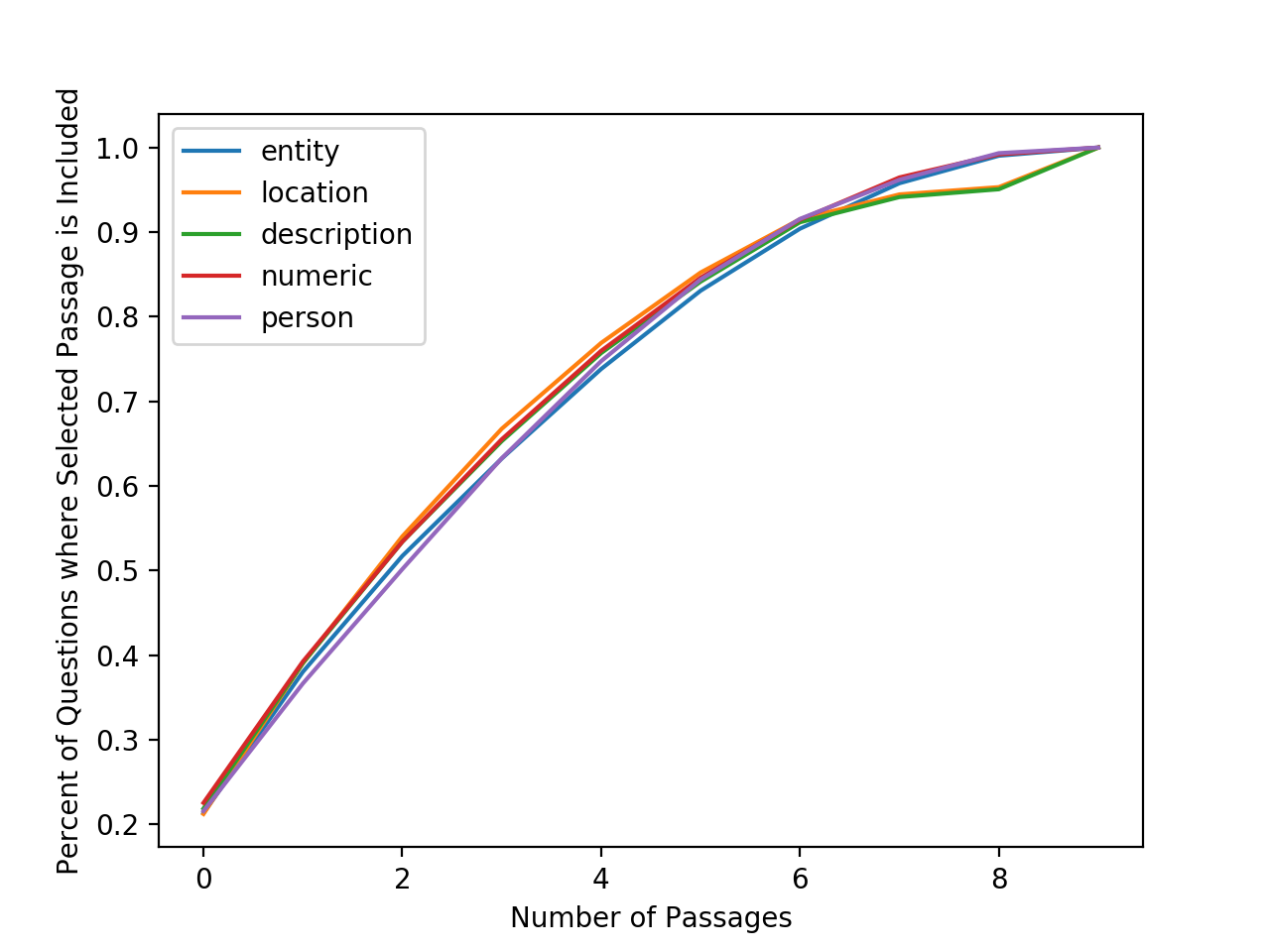
The graph above shows the percent of questions for which the selected passage appears in the top n highest ranked passages. Using this, we can decide how many passages we must include to achieve a certain accuracy.
Question type does not have a noticeable effect on accuracy, except for when most passages are included, when the location and description types have somewhat lower accuracy than other question types.
We had hoped that it would be possible to achieve high accuracy even when including just a few passages. Unfortunately, this does not seem possible with the current model. There are numerous tweaks that we could explore to boost this accuracy. For example, we could explore different kernels and similarity metrics.
Another important question is how important is it that we find the selected passage? Can we still achieve high Bleu scores by using passages that the reference did not use? I suspect that we could do quite well for question types with short answers when not using the passage that the reference used. For example, the answer to the location question “at what russian city on the volga did the germans suffer a major defeat” is “Stalingrad”. This question could be answered by looking at any of the provided passages, not just the selected one.
Next Steps
Now that we have the passages ranked, the question is how to passage them through the model and get the answer? One initially proposed method would be, with the ranked documents, pass each one through the answer extractor individually, which gives us numerous individual answers. From there, we would need to assign weights to each of the answers based on how the passages were ranked initially. Instead of just taking the answer from the highest ranked passage, we want to find a way to measure the similarities between the various answers. If there is an answer that appears multiple times, then we would want to add the weights of these answers together and merge them into a single answer. Finally, pick the answer that has the highest weight.
For the upcoming week, we will work on creating the pipeline to do this, as well as experiment with similarity metrics to cluster the answers after they have been passage through the model.